Table of contents

1. 2018.11.29 Testing Intel RealSense using pyRealSense
2. 2018.11.28 Testing Intel RealSense using librealsense
3. 2018.09.21 Thesis defense
4. 2018.07.24 Final deposit of the thesis
5. 2018.07.01-20 Thoroughly reviewing thesis document for final deposit
6. 2018.06.15-27. Reviewing and translating thesis document into English to deposit draft version
7. 2018.06.08. New experiments with US, IR and camera sensors
   1. PiBot bump and go using ultrasonic sensor
   2. PiBot follow line using infrared sensor
   3. PiBot follow line using vision
8. 2018.06.05. First version of Chapter 4. Teaching Robotics framework
9. 2018.05.29. First version of Chapter 3. Robots with vision
10. 2018.05.22. First version of Chapter 2. State of art
11. 2018.05.15. First version of Chapter 5. Conclusions
12. 2018.05.08. First version of Chapter 1. Introduction
13. 2018.05.06. Demonstrating new version features of the visual sonar system
14. 2018.05.05. New version of the visual sonar system
15. 2018.05.02. Avoiding obstacles using visual sonar and benchmark
16. 2018.05.01. Vision system robustness tests
17. 2018.04.30. New enriched 3D visualizer using PyGame library
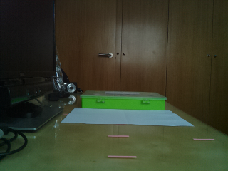
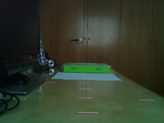
18. 2018.04.21. Right Ground frontier 3D points
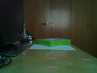
19. 2018.04.18. Wrong Ground frontier 3D points
20. 2018.04.15. Frontier image filtered
21. 2018.04.10. Show camera extrinsic parameters in a 3D Scene
22. 2018.04.08. Back-projecting pixels to 3D
23. 2018.04.06. Modeling the scene
24. 2018.03.31. Pin-Hole camera model class
25. 2018.03.21. Calibrating PiCam
    1. Intrinsic parameters
    2. Extrinsic parameters
    3. PiCam calibration app
26. 2018.03.17. Reviewing vision concepts
    1. Pin-Hole camera model
    2. Epipolar Geometry
    3. Ground hypothesis
    4. Homogeneous image coordinates
    5. Using matrices to save camera position
       1. Introduction
       2. Using matrices
       3. Expressing camera position as Position + FOA (Focus Of Attention)
27. 2018.03.08. Starting from scratch with the new FeedBack 350º Servos
28. 2018.03.03. Introducing the new PiBot v3.0
29. 2018.03.01. JdeRobot-Kids as a multiplatform Robotics middleware
30. 2018.02.18. PiBot following a blue ball
31. 2018.02.11. PiBot v2.0 (full equipment) working
32. 2018.02.10. New design of the PiBot v2.0 (full equipment) for using JdeRobot-Kids API
33. 2018.02.09. Testing how to define and use abstract base classes for JdeRobot-Kids API
34. 2018.02.08. Introducing the new robotic platform: piBot
35. 2018.02.04. New device supported on Raspberry Pi 3: RC Servo
36. 2018.02.01. New sensor supported on Raspberry Pi 3: Ultrasonic
37. 2018.01.27. New PiCam ICE-driver developed
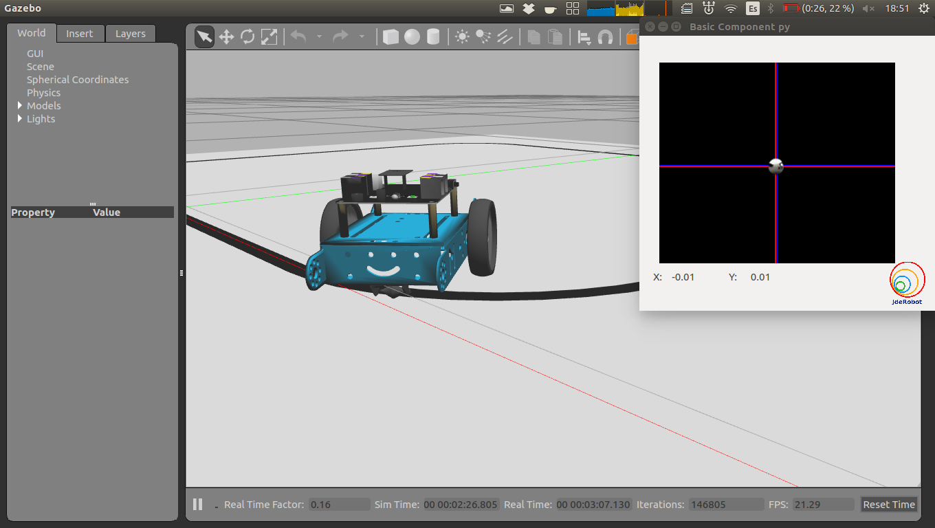
38. 2018.01.23. Testing plug-in mBot under gazeboserver using a basic COMM tool
39. 2018.01.13. New ball tracking: suitable for ICE and COMM communications
40. 2018.01.06. Ball tracking using Python and OpenCV

2018.11.29 Testing Intel RealSense using pyRealSense

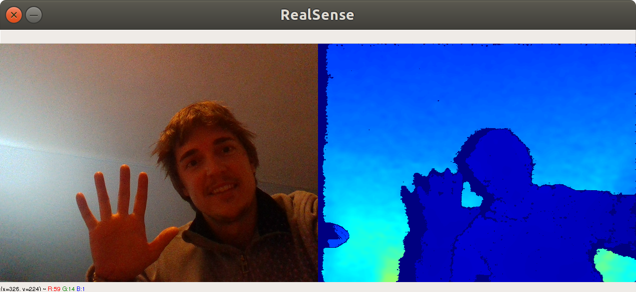
2018.11.28 Testing Intel RealSense using librealsense

2018.09.21 Thesis defense

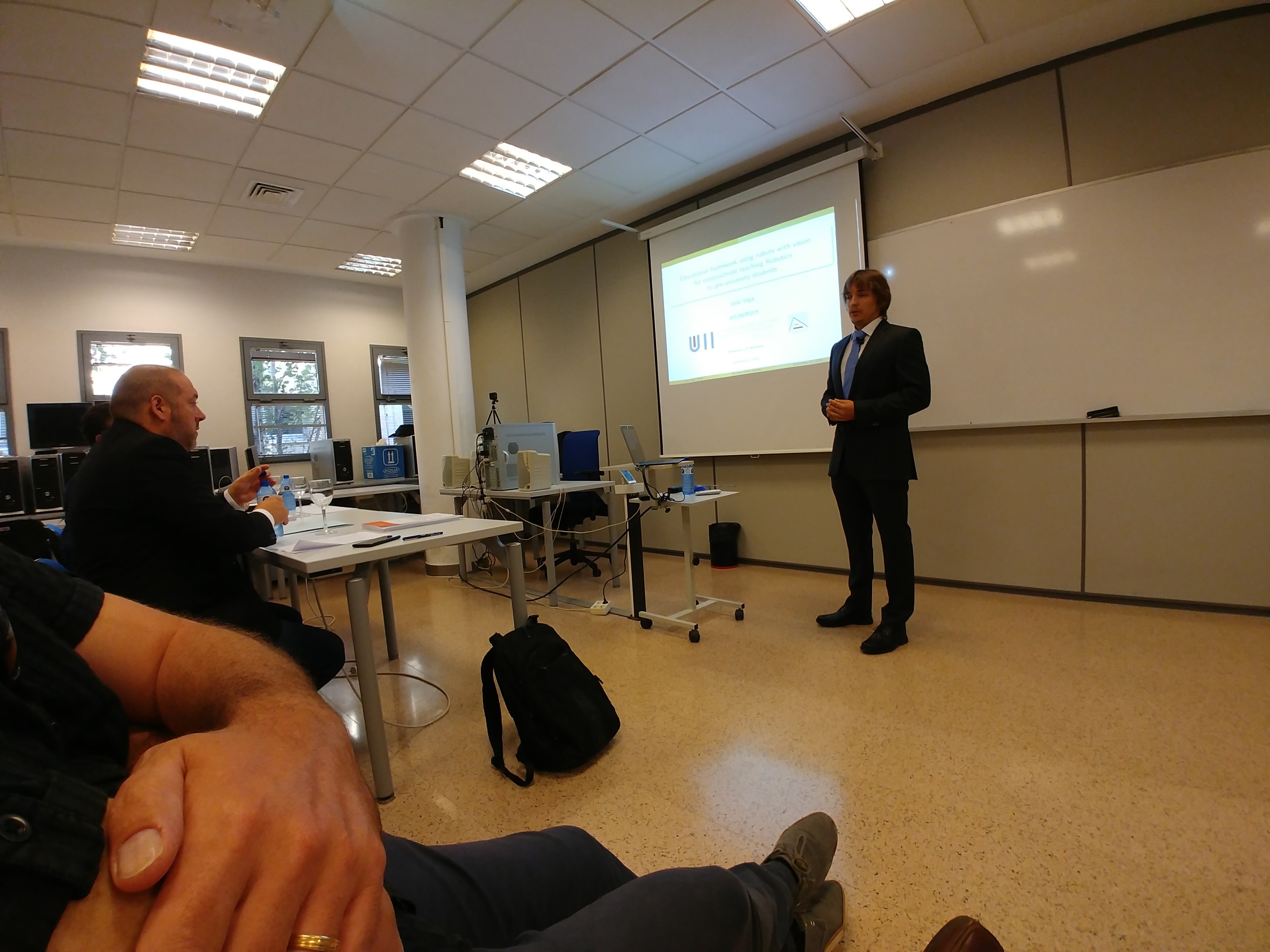
The slides are available here

2018.07.24 Final deposit of the thesis

The document is available here

2018.07.01-20 Thoroughly reviewing thesis document for final deposit

2018.06.15-27. Reviewing and translating thesis document into English to deposit draft version

2018.06.08. New experiments with US, IR and camera sensors

PiBot bump and go using ultrasonic sensor

PiBot follow line using infrared sensor

PiBot follow line using vision

2018.06.05. First version of Chapter 4. Teaching Robotics framework

2018.05.29. First version of Chapter 3. Robots with vision

2018.05.22. First version of Chapter 2. State of art

2018.05.15. First version of Chapter 5. Conclusions

2018.05.08. First version of Chapter 1. Introduction

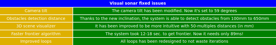
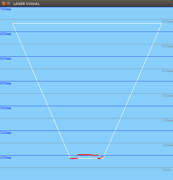
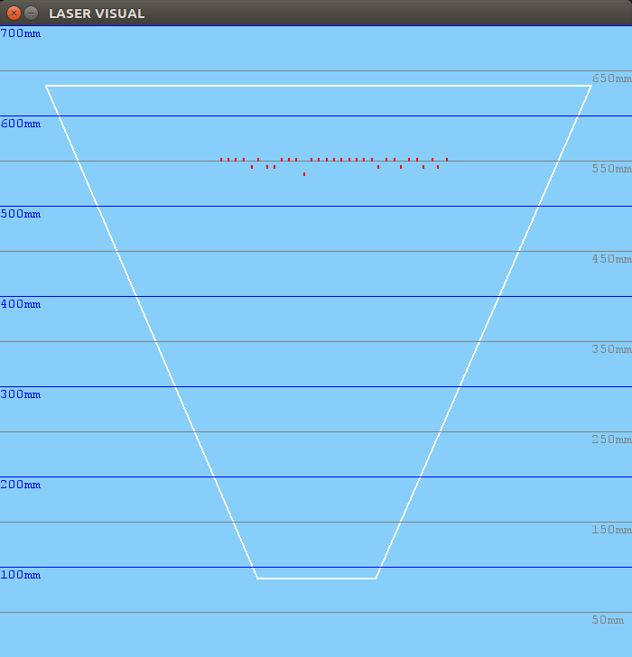
2018.05.06. Demonstrating new version features of the visual sonar system

As we can see on this video, the robot is closer to the obstacles than last time. This is because of the new tilt angle which lets robot detect obstacle from 90mm to 650mm. Previously, the closest obstacle it could detect was 250mm.

Furthermore, the system is faster, taking only 89ms to get frontier.

2018.05.05. New version of the visual sonar system

A new version of the visual sonar has been developed in order to fix some issues:

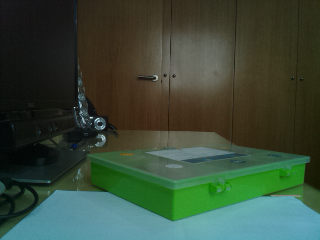
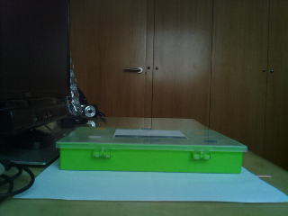
Here we can see the aspect of the new PiBot with the camera tilt inclined:

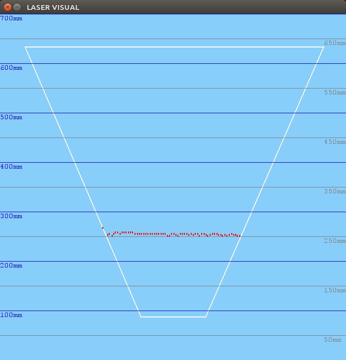
And it has been tested successfully. Here we see some examples:

100mm distance:

250mm distance:

400mm distance:

550mm distance:

2018.05.02. Avoiding obstacles using visual sonar and benchmark

On this video we are using the visual sensor, the PiCam, to avoid green obstacles. We consider obstacles are on the floor, thus, we can estimate distances using a single camera, matching optical rays with ground plane (Z = 0). In this case, the system intersects rays with the obstacle frontier previously got as following: original image -> rgb filter -> hsv filter -> green filter -> frontier own algorithm -> backproject frontier -> frontier 3D memory -> calculate min distance to it.

Once we have benchmarked the system, we get the following timing:

1st. Load Pin Hole camera model: 0.5 ms

2nd. Initialize PiCam: 0.5 s

3rd. Filter image till getting B/W obstacles filtered: 35 ms

4th. Get 2D frontier and backproject it onto the ground: 12 - 18 s

5th. Get min distance to 3D frontier and command motors properly: 0.5 s

So, as we can see and we could guess, the hard process is getting the 2D frontier and backproject it to the 3D ground.

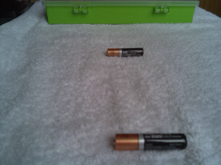
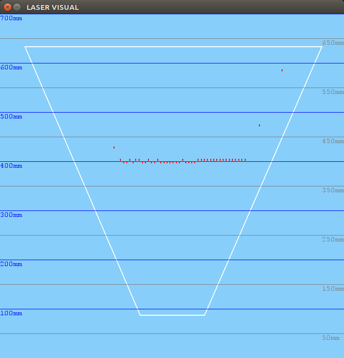
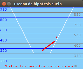
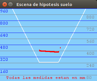
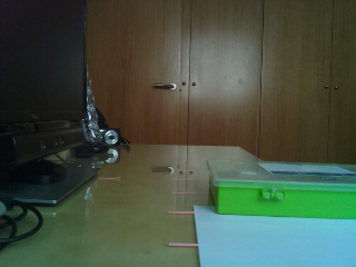
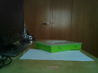
2018.05.01. Vision system robustness tests

After arranging several issues about the translation between the different coordinate systems we have in our vision system: optical system, world system and virtual representation system (PyGame) with an scaled world, we have tested the robustness of the system through a series of images with objects placed at different distances exactly measured. The results are plausible:

300mm distance:

400mm distance:

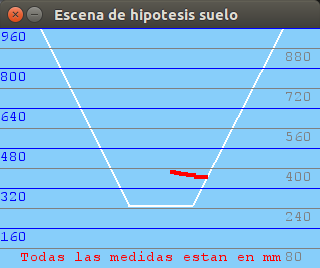
500mm distance:

600mm distance:

700mm distance:

900mm distance:

2018.04.30. New enriched 3D visualizer using PyGame library

The library PyGame is a Free and Open Source Python programming language library for making multimedia applications like games built on top of the excellent SDL library. Like SDL, pygame is highly portable and runs on nearly every platform and operating system.

We use it because it offers simple functions to draw lines, circles (points) and it runs with its own graphic engine. It's so light, ideal for the Raspberry Pi.

So, the new aspect of the 3D scene visualizer results in a colorful, intuitive and friendly window:

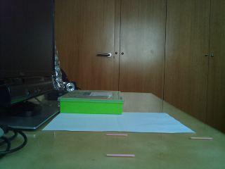
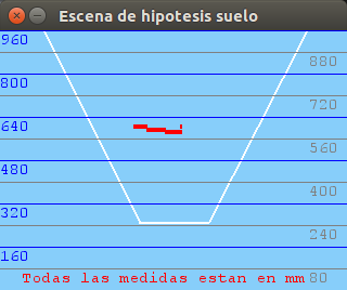
2018.04.21. Right Ground frontier 3D points

After a re-calibrate process, setting correctly some camera parameters and doing a deep effort to translate properly from a image pixel to backproject it and then translate it to another coordinate system in order to draw the world over a simple 2D images, we finally get a right ground frontier 3D points, which we can see on the next figure. We consider 1 pixel on the figure corresponds to 1 mm on the real world.

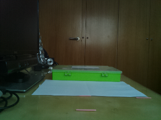
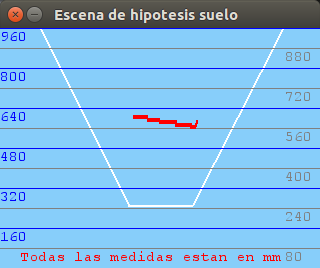
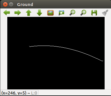
2018.04.18. Wrong Ground frontier 3D points

After getting the frontier filtered points we can see in the last post, they are back-projected onto the ground floor, because we are assuming that objects (obstacles) are in Z = 0 plane. Following the Pin-hole camera model we designed for the PiCam, which includes several matrix operations and projective geometry techniques, we finally get the picture. It includes the 3D resultant ground-points (Z = 0), but the camera lens model must need some re-adjustment, probably it has to be with distortion parameters, which we assumed 0. To be continued...

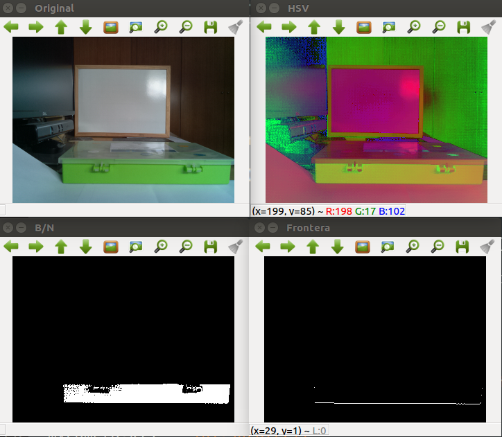
2018.04.15. Frontier image filtered

The original image got from the PiCam is filtered to HSV scale, then an hsv-color filter is applied to get green obstacles filtered and shown in a black and white which it is tracked in a columns bottom-up algorithm, where each pixel is evaluated with respect to its eight neighbors, to see whether it is a border point between ground and object (assuming is on the ground) or not.

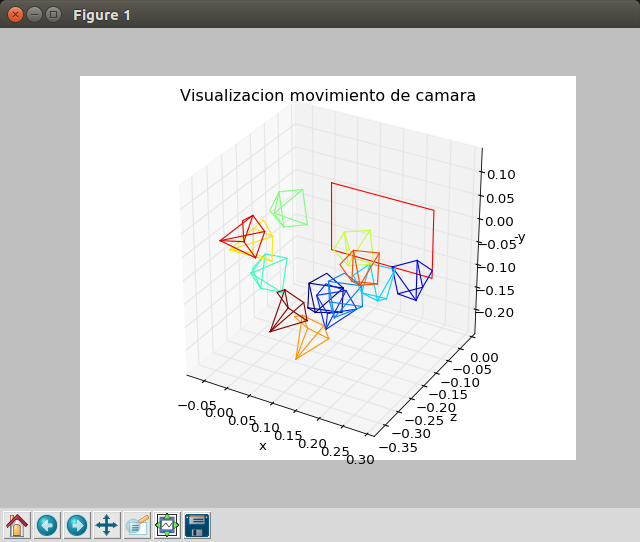
2018.04.10. Show camera extrinsic parameters in a 3D Scene

In order to visualize the camera extrinsic parameters, despite we have no controlled motor-encoders yet, a 3D plotter has been developed. With this tool we can load a simulation of camera movements through coordinates introduced manually on a configuration file, and we can see the 3D scene rendered with the different camera poses. The board represents the chess board which we used to calibrate the PiCam.

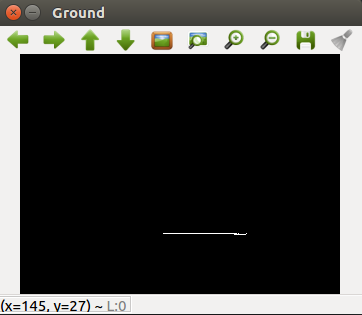
2018.04.08. Back-projecting pixels to 3D

We achieved back-project 2D to 3D pixels using our Pin-hole camera class and some OpenCV functions to draw the back-projection line. We get the first black pixel below the image to estimate depth. The result is as following.

2018.04.06. Modeling the scene

We have introduced a 3D scene renderer under OpenGL in our purpose of showing a full camera model with the ray-tracing got from the objects surrounding the robot.

Our first purpose is to develop a visual-sonar to design a complete navigation algorithm avoiding obstacles using a single sensor: vision.

But, after several tries, we observe OpenGL was so complex, so we changed to use OpenCV drawing functions.

2018.03.31. Pin-Hole camera model class

We have been developing a new class for JdeRobot-Kids middleware, called "PinholeCamera.py". It includes all necessary methods to work with a Pin-hole camera model as well as matrices. The class doc is attached below:

NAME
    PinholeCamera

FILE
    /JdeRobot-Kids/visionLib/PinholeCamera.py

DESCRIPTION
    ###############################################################################
    # En este fichero se implementa la clase correspondiente a una camara modelo  #
    # Pin Hole, o camara ideal. Los parametros para el manejo de una camara       #
    # y la calibracion de esta se recogen en las matrices K, R, P (incluye T) que,#
    # inicialmente seran 0 (antes de efectuar la calibracion)                     #
    ###############################################################################
    # Matrices o parametros de calibracion:
    # A) Image sin distorsionar: requiere D y K
    # B) Imagen rectificada: requiere D, K y R
    ##############################################################################
    # Dimension de las imagenes de la camara; normalmente es la resolucion (en 
    # pixels) de la resolucion de la camara: height y width
    ##############################################################################
    # Descripcion de las matrices:
    # Matriz de parametros intrinsecos (para imagenes distorsionadas)
    #     [fx  0 cx]
    # K = [ 0 fy cy]
    #     [ 0  0  1]
    # Matriz de rectificacion de camara (rotacion): R
    # Matriz de proyeccion o matriz de camara (incluye K y T)
    #     [fx'  0  cx' Tx]
    # P = [ 0  fy' cy' Ty]
    #     [ 0   0   1   0]
    ##############################################################################

CLASSES
    PinholeCamera
    
    class PinholeCamera
     |  Una camara modelo Pin Hole es una camara ideal.
     |  
     |  Methods defined here:
     |  
     |  __init__(self)
     |  
     |  getCx(self)
     |  
     |  getCy(self)
     |  
     |  getD(self)
     |  
     |  getFx(self)
     |  
     |  getFy(self)
     |  
     |  getK(self)
     |  
     |  getP(self)
     |  
     |  getR(self)
     |  
     |  getResolucionCamara(self)
     |  
     |  getTx(self)
     |  
     |  getTy(self)
     |  
     |  getU0(self)
     |  
     |  getV0(self)
     |  
     |  proyectar3DAPixel(self, point)
     |      :param point:     punto 3D
     |      :type point:      (x, y, z)
     |      Convierte el punto 3D a las coordenadas del pixel rectificado (u, v),
     |      usando la matriz de proyeccion :math:`P`.
     |      Esta funcion es la inversa a :meth:`proyectarPixelARayo3D`.
     |  
     |  proyectarPixelARayo3D(self, uv)
     |      :param uv:        coordenadas de pixel rectificadas
     |      :type uv:         (u, v)
     |      Devuelve el vector unidad que pasa por el centro de la camara a traves 
     |      del pixel rectificado (u, v), usando la matriz de proyeccion :math:`P`.
     |      Este metodo es el inverso a :meth:`proyectar3DAPixel`.
     |  
     |  rectificarImagen(self, raw, rectified)
     |      :param raw:       input image
     |      :type raw:        :class:`CvMat` or :class:`IplImage`
     |      :param rectified: imagen de salida rectificada
     |      :type rectified:  :class:`CvMat` or :class:`IplImage`
     |      Aplica la rectificacion especificada por los parametros de camara 
     |      :math:`K` y :math:`D` a la imagen `raw` y escribe la imagen resultante 
     |      en `rectified`.
     |  
     |  rectificarPunto(self, uv_raw)
     |      :param uv_raw:    coordenadas del pixel
     |      :type uv_raw:     (u, v)
     |      Aplica la rectificacion especificada por los parametros de camara
     |      :math:`K` y :math:`D` al punto (u, v) y retorna las coordenadas del
     |      pixel del punto rectificado.
     |  
     |  setPinHoleCamera(self, K, D, R, P, width, height)

FUNCTIONS
    construirMatriz(rows, cols, L)

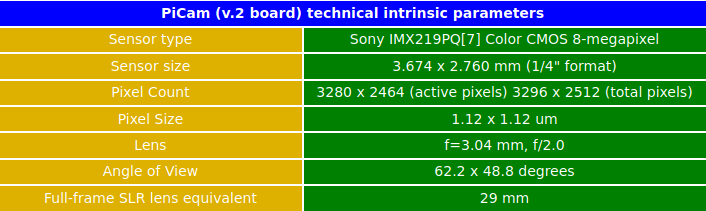
2018.03.21. Calibrating PiCam

Intrinsic parameters

According to the manufacturer's manual, the PiCam (v2.1 board) technical intrinsic parameters are as following:

Extrinsic parameters

PiCam calibration app

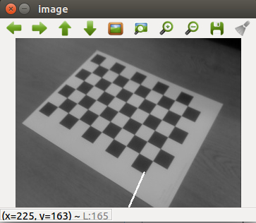
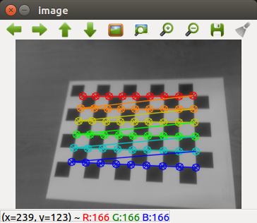
Despite having the intrinsic parameters provided by the manufacturer, and since not all cameras have the same factory calibration, we have developed an app called PiCamCalibration.py to get these values. It uses several OpenCV functions to get the K matrix finally.

Firstly we goty 10 test patterns for camera calibration using a chess board. To find pattern in chess board we use the function cv2.findChessboardCorners() and to draw the pattern we use cv2.drawChessboardCorners() as we can see in the next figure.

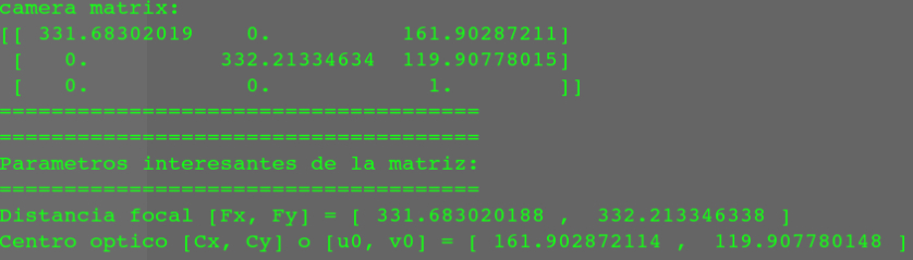
So now we have our object points and image points we are ready to go for calibration. For that we use the function cv2.calibrateCamera(). It returns the camera matrix, distortion coefficients, rotation and translation vectors etc.

We show an screen-shot below of the output of our software.

2018.03.17. Reviewing vision concepts

We want PiBot to support vision algorithms using the single PiCam camera on board. That's why, we need to introduce some advanced concepts in Geometry.

Pin-Hole camera model

Firstly, the camera model needs to be implemented. The camera model we are going to use is an ideal camera, called Pin-hole camera. When we take an image using a pin-hole camera, we loose an important information, i.e. depth of the image. Or even how far is each point in the image from the camera, because it is a 3D-to-2D conversion. So it is an important question whether we can find the depth information using cameras. And the answer is to use more than one camera. Our eyes works in similar way where we use two cameras (two eyes) which is called stereo vision. And OpenCV provides lots of useful functions in this field.

The image below shows a basic setup with two cameras taking the image of same scene (from OpenCV).

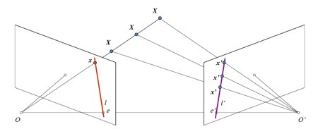
Epipolar Geometry

As we are using a single camera, we can’t find the 3D point corresponding to the point x in image because every point on the line OX projects to the same point on the image plane. With two cameras we get these two images and we can triangulate the correct 3D point. In this case, to find the matching point in other image, you don't need to search the whole image, but along the epiline. This is called Epipolar Constraint. Similarly all points will have its corresponding epilines in the other image. The plane XOO' is called Epipolar Plane.

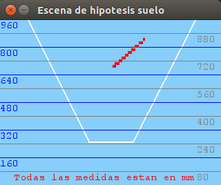
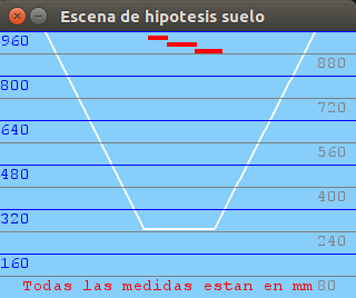
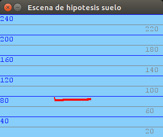
Ground hypothesis

If we want to estimate distances from the robot to the surrounding objects, the key question is how can I get a depth map with a single camera? Or, in other words, how can I find the 3D point corresponding to the point x in the image above with a single camera?

To do that, and following the Ground Hypothesis, we consider that all the objects are on the floor, on the ground plane, which we know where is (on plane Z = 0). That way, we can find the 3D point corresponding to every point in the single image, as we can see in the image below.

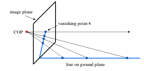
So, if we get the pixels corresponding to the filtered border below the obstacles we can get the distance to them.

Homogeneous image coordinates

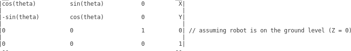
To compute the rays back-projecting those pixels, the position of the camera needs to be calculated. A camera is defined and positioned according to its matrices K * R * T, where:

- K (3x3) = intrinsic parameters

- R (3x3) = camera rotation

- T (3x1) = translation vector of the camera in X, Y, Z:

- X = forward movement

- Y = shift to the left

- Z = upward movement

(always looking from the point of view of what we are moving)

Also, we can use a single matrix that includes RT, and would therefore be 4x4, as we see below. They always follow the same form.

So, given a point in ground plane coordinates Pg = [X, Y, Z], its coordinates in camera frame (Pc) are given by:

Pc = R * Pg + t

The camera center is Cc = [0, 0, 0] in camera coordinates. In ground coordinates it is then:

Cg = -R' * t, where R' is the transpose of R.

(Assuming, as we saw before, for simplicity, that the the ground plane is Z = 0.)

Let K be the matrix of intrinsic parameters (we will see proximately). Given a pixel q = [u, v], write it in homogeneous image coordinates Q = [u, v, 1]. Its location in camera coordinates (Qc) is:

Qc = Ki * Q

where Ki = inv(K) is the inverse of the intrinsic parameters matrix. The same point in world coordinates (Qg) is then:

Qg = R' * Qc -R' * t

All the points Pg = [X, Y, Z] that belong to the ray from the camera center through that pixel, expressed in ground coordinates, are then on the line

Pg = Cg + theta * (Qg - Cg)

(for theta going from 0 to positive infinity.)

Using matrices to save camera position

Introduction

If we have the camera moved with respect to several axes, we must multiply the matrices one by another, once and again. For example, for a complete translation of the camera:

1st. If we have encoders with information of X, Y and Theta, the robot is moved with respect to the absolute (0, 0) of the world, and rotated with respect to the Z axis, so the RT matrix of the robot would be:

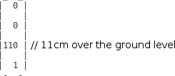
2nd. If we have a Pan-Tilt unit for the camera, it will be moved with respect to the base of the robot (which is on the ground level).

3rd. The Tilt axis is translated in Z with respect to the base of the Pan-Tilt, and rotated with respect to the Z axis according to Pan angle.

4th. The Tilt axis is also rotated with respect to the Y axis according to the Tilt angle.

5th. The optical center of the camera is translated in X and in Z with respect to the Tilt axis.

Using matrices

To obtain the absolute position of the camera in the world we multiply the previous matrices as following:

temp1 = 1st * 2nd

temp2 = temp1 * 3rd

temp3 = temp2 * 4th

temp4 = temp3 * 5th

We already have got in temp4 [0,3] [1,3] [2,3] the absolute position X, Y, Z of the camera.

Expressing camera position as Position + FOA (Focus Of Attention)

If we express the camera as "POSITION + FOA" we will have to add to the previous resultant matrix ("temp4") the relative FOA of the camera, which is saved in a 4x1 vector. For example, if "relativeFOA" is:

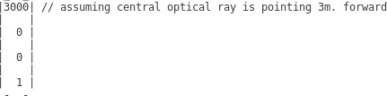
Then, the absolute FOA will be expressed (and saved) in a 4x1 vector ("absoluteFOA") according to:

absoluteFOA = temp4 * relativeFOA

2018.03.08. Starting from scratch with the new FeedBack 350º Servos

I connect the servos correctly; the servo requires an input control signal sent from the microcontroller via the white wire connection. But, what I can't, is reading the feedback information properly.

Following the manufacturer's manual, the servo sends a feedback output signal to your microcontroller via the yellow wire connection. This signal, labeled tCycle in the diagrams and equations below, has a period of 1/910 Hz (approx. 1.1 ms), +/- 5%.

Within each tCycle iteration, tHigh is the duration in microseconds of a 3.3 V high pulse. The duration of tHigh varies with the output of a Hall-effect sensor inside of the servo. The duty cycle of this signal, tHigh / tCycle, ranges from 2.9% at the origin to 97.1% approaching one clockwise revolution.

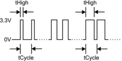
Duty cycle corresponds to the rotational position of the servo, in the units per full circle desired for the application.

For example, a rolling robot application may use 64 units, or “ticks” per full circle, mimicking the behavior or a 32-spoke wheel with an optical 1-bit binary encoder. A fixed-position application may use 360 units, to move and hold the servo to a certain angle.

The following formula can be used to correlate the feedback signal’s duty cycle to angular position in your chosen units per full circle.

Duty Cycle = 100% x (tHigh / tCycle). Duty Cycle Min = 2.9%. Duty Cycle Max= 97.1%.

(Duty Cycle - Duty Cycle Min) x units full circle

Angular position in units full circle = _________________________________________________________________________________

Duty Cycle Max - Duty Cycle Min + 1

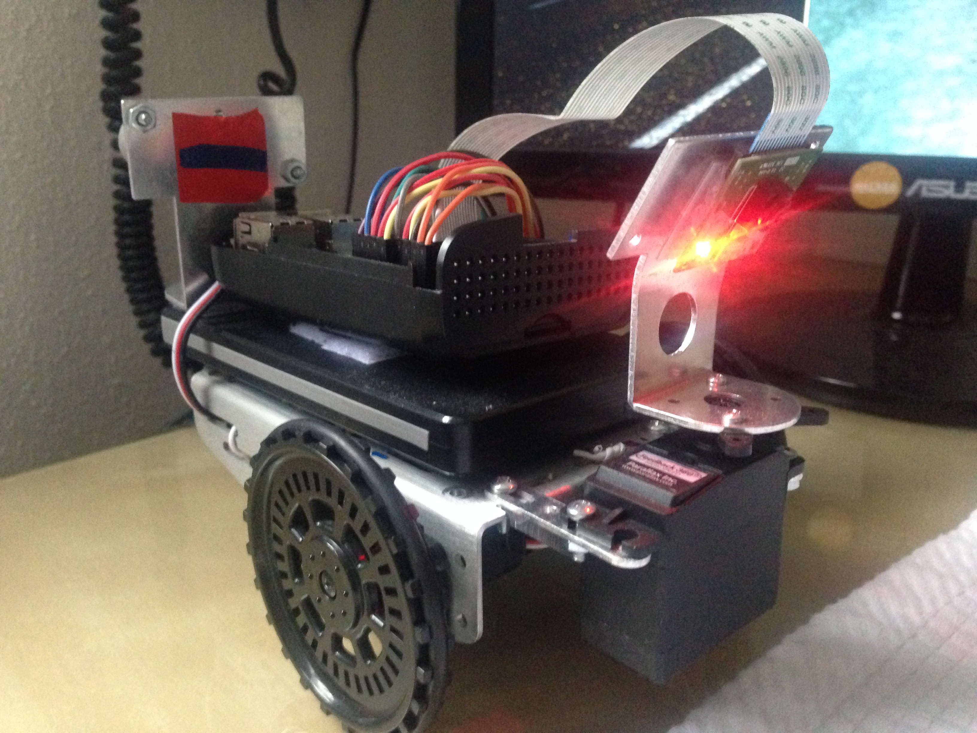
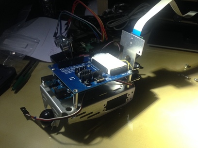
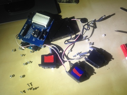
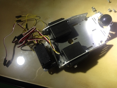
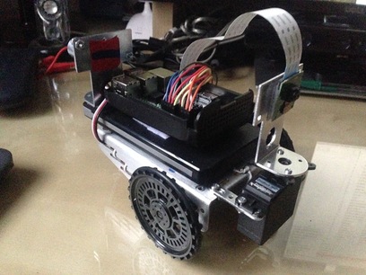
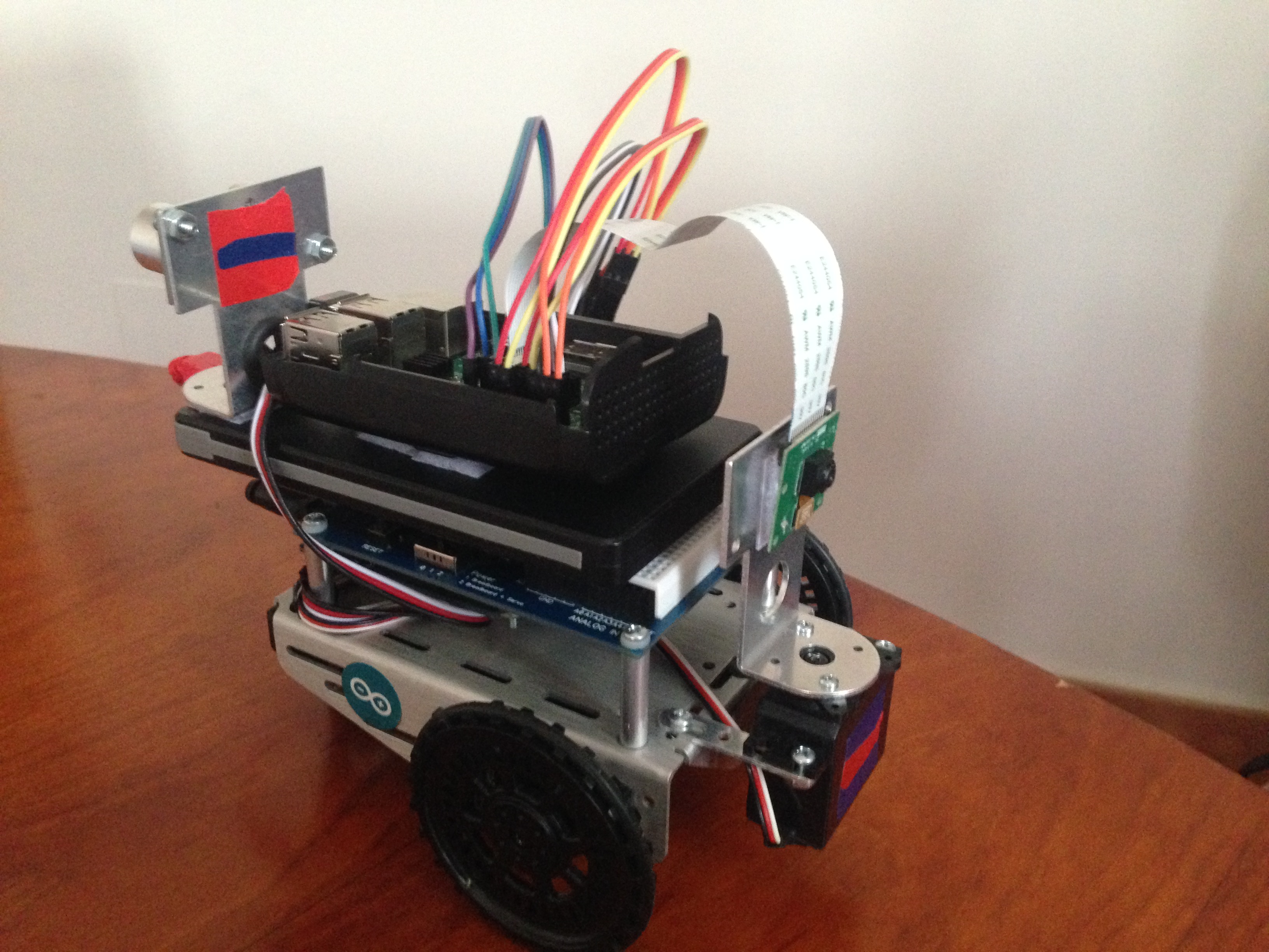
2018.03.03. Introducing the new PiBot v3.0

I've started from scratch with the PiBot prototype in order to add the new FeedBack 350º Servos (by Parallax) which include encoders.

The following shows the design process described with images.

First steps: removing all components

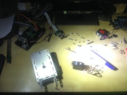
Adding new Servos and wheels on board

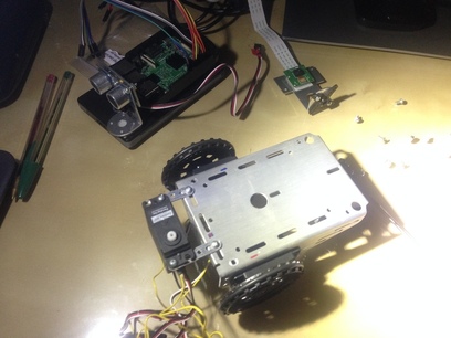
Last steps: Mounting Battery, PiCam and Raspberry Pi 3, hiding tedious cables and weighting it

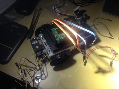
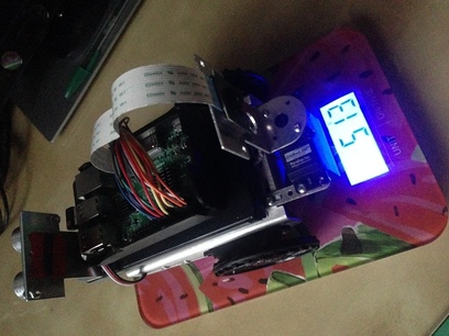
Result: the new PiBot v3.0

2018.03.01. JdeRobot-Kids as a multiplatform Robotics middleware

On this video we can see an example of how we can use JdeRobot-Kids with different robotic platforms, such as mBot real or Gazebo-simulated, and piBot (Raspberry Pi Robot).

We just need to change the robot platform field in the configuration file and the application (written in Python language) over JdeRobot-Kids middleware, will work in the same way for all the platforms described previously.

2018.02.18. PiBot following a blue ball

We have developed a new algorithm called "FollowBall". It extracts a filtered colored object, gets its position and then it applies a PID controlled algorithm in order to manage properly the two motors. The goal is to properly guide the direction of the robot to keep the pursued object in the center of the current frame at all times.

2018.02.11. PiBot v2.0 (full equipment) working

On this video, we can see the PiBot v2.0 (full equipment) working. It is equiped with an ultrasonic sensor, two continuous servos to drive left and right wheels, and a turret-PiCamera mounted on a 180º simple servo.

This way we have already reached the limit of voltage pins, since we have used the four voltage pins (2x5V + 2x3.3V) that Raspberry Pi3 has available, although there are many other more GPIO pins.

2018.02.10. New design of the PiBot v2.0 (full equipment) for using JdeRobot-Kids API

We have been designing and making the new PiBot model to take advantage of the JdeRobot-Kids infrastructure and have a fully functional robot. We run into the limitation of the four voltage pins available in the Raspberry Pi3.

It is equiped with an ultrasonic sensor, two continuous servos to drive left and right wheels, and a turret-PiCamera mounted on a 180º simple servo.

2018.02.09. Testing how to define and use abstract base classes for JdeRobot-Kids API

Our purpose is to develop the next schema, using JdeRobot-Kids on the top level as an abstract class called "JdeRobotKids.py", which is the common API for young students, and it is defined in a set of subclasses: "mBotReal", "mBotGazebo" and "piBot". This library is used by the user, through his/her own code in a python file (e.g. "myAlgorithm.py").

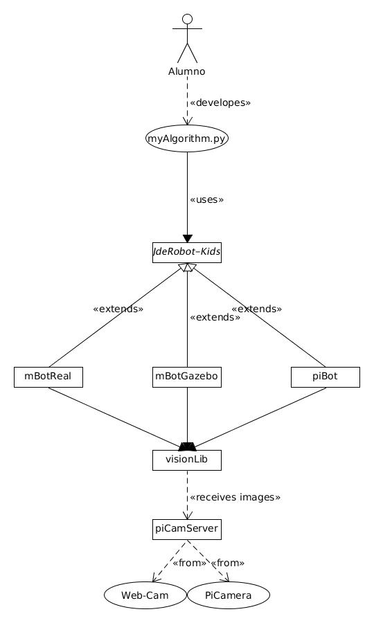
That's why we have started testing simple classes using the "abc" library (Abstract Base Classes). It works by marking methods of the base class as abstract, and then registering concrete classes as implementations of the abstract base.

This example code can be downloaded from here

(Bonus track) If you need to include the import files in different folders, you cant't (by default) because Python only searches the current directory, the directory that the entry-point script is running from. However, you can add to the Python path at runtime:

import sys
sys.path.insert(0, './mBotReal')
sys.path.insert(0, './mBotGazebo')
sys.path.insert(0, './piBot')

2018.02.08. Introducing the new robotic platform: piBot

On this video we introduce the new robotic platform, which we've called piBot because it uses the Raspberry Pi as a main-board instead of Arduino.

As we can see, we control two continuous rotation servos using a wireless USB keyboard through the Raspberry Pi, using the GPIO ports and coded in Python.

2018.02.04. New device supported on Raspberry Pi 3: RC Servo

This new device, a RC 180 degrees servo, has been programmed in Python language and as we can see on this video it's able to move from the center position (90 degrees) to 0 and 180 degrees (approximately), using the Raspberry Pi 3 GPIO ports.

2018.02.01. New sensor supported on Raspberry Pi 3: Ultrasonic

We have adapted the ultrasonic sensor through electronics to be supported by the GPIO ports of the raspberry pi 3. Using an application written in Python we can read the values sensed by this sensor.

The output signal of this sensor is rated at 5V, but the input GPIO-pin on the Raspberry is rated at 3.3V. So, sending a 5V signal into a 3.3V input port could damage the Raspberry card or, at least, this pin. That's why we've implemented a voltage divider circuit with two resistors in order to lower the sensor output voltage to our Raspberry Pi GPIO port.

We can see the results on the next video:

2018.01.27. New PiCam ICE-driver developed

We have developed a new driver, called PiCamServer, which supports the Raspberry Pi 3 camera (a.k.a. PiCam). This driver is a server which serves images through ICE communications.

On the next video, we can see how the new driver can serve images from a webcam or a PiCam, just changing the device in the server configuration file, so that we can get these images using a simple images-client tool under ICE protocol.

2018.01.23. Testing plug-in mBot under gazeboserver using a basic COMM tool

We can command a Gazebo-simulated mBot robot using a COMM communications between gazeboserver and a basic written-in-Python Qt tool.

2018.01.13. New ball tracking: suitable for ICE and COMM communications

We have improved the compatibility of our application in order to get images from a ICE or COMM server, which let it communicate with ROS and JdeRobot middle-wares.

Furthermore, the behavior of our algorithm has been also customized for getting the maximum colored object. We can see how it works with two similar objects in this video.

2018.01.06. Ball tracking using Python and OpenCV

Once we know how to convert BGR image to HSV, we can use this to extract a colored object. In HSV, it is easier to represent a color than in RGB color-space. In our application, we extract a blue colored object. The method is as following:

- Take each frame of the video.

- Convert from BGR to HSV color-space.

- We threshold the HSV image for a range of blue color.

- Now extract the blue object alone, we can do whatever on that image we want.

We can see the result in this video. The output indicates the ball position in every moment.